2014_militrary_expenditures_absolute.svg

Size of this PNG preview of this SVG file:
512 × 288 pixels
.
Other resolutions:
320 × 180 pixels
|
640 × 360 pixels
|
1,024 × 576 pixels
|
1,280 × 720 pixels
|
2,560 × 1,440 pixels
.
Summary
| Description |
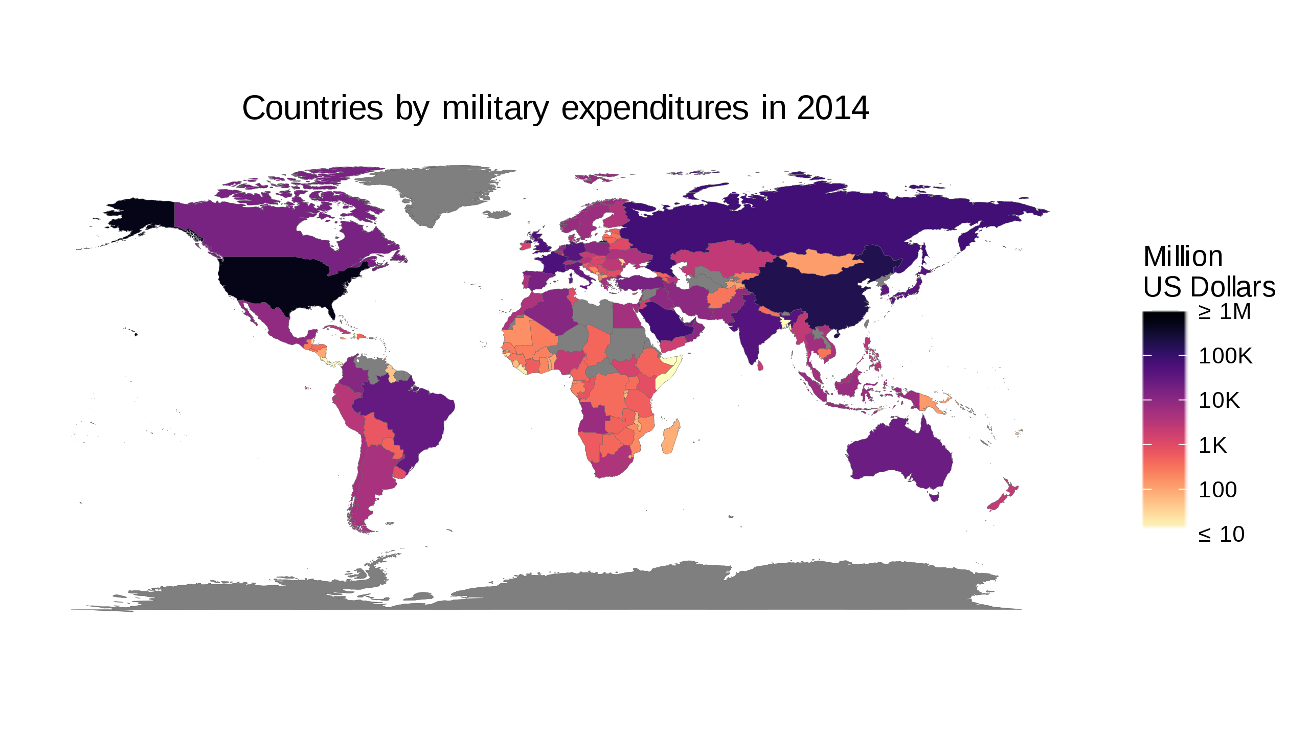
English:
Based on the Worldbank data from
http://data.worldbank.org/indicator/MS.MIL.XPND.GD.ZS
and
http://data.worldbank.org/indicator/NY.GDP.MKTP.CD
This is a candidate for replacing/augmenting
https://commons.wikimedia.org/wiki/File:Countries_by_Military_expenditures_(%25_of_GDP)_in_2014_v2.svg
|
| Source | Own work |
| Author | Pipping |
_in_2014_v2.svg)
Licensing
I, the copyright holder of this work, hereby publish it under the following license:
This file is licensed under the
Creative Commons
Attribution-Share Alike 4.0 International
license.
-
You are free:
- to share – to copy, distribute and transmit the work
- to remix – to adapt the work
-
Under the following conditions:
- attribution – You must give appropriate credit, provide a link to the license, and indicate if changes were made. You may do so in any reasonable manner, but not in any way that suggests the licensor endorses you or your use.
- share alike – If you remix, transform, or build upon the material, you must distribute your contributions under the same or compatible license as the original.
Created with the following piece of code:
library(magrittr)

selectedYear <- 2014

getWorldBankData <- function(indicatorCode, indicatorName) {
    baseName <- paste('API', indicatorCode, 'DS2_en_csv_v2', sep='_')
    ## Download zipfile if necessary
    zipfile <- paste(baseName, 'zip', sep='.')
    if (!file.exists(zipfile)) {
        zipurl <- paste(paste('http://api.worldbank.org/v2/en/indicator',
                              indicatorCode, sep='/'),
                        'downloadformat=csv', sep='?')
        download.file(zipurl, zipfile)
    }
    csvfile <- paste(baseName, 'csv', sep='.')
    ## This produces a warning because of the trailing commas. Safe to ignore.
    readr::read_csv(unz(zipfile, csvfile), skip=4,
                    col_types = list(`Indicator Name` = readr::col_character(),
                                     `Indicator Code` = readr::col_character(),
                                     `Country Name` = readr::col_character(),
                                     `Country Code` = readr::col_character(),
                                     .default = readr::col_double())) %>%
        dplyr::select(-c(`Indicator Name`, `Indicator Code`, `Country Name`))
}

## Obtain and merge World Bank data
worldBankData <-
    dplyr::left_join(
               getWorldBankData('MS.MIL.XPND.GD.ZS') %>%
               tidyr::gather(-`Country Code`, convert=TRUE,
                             key='Year', value=`Military expenditure (% of GDP)`,
                             na.rm = TRUE),
               getWorldBankData('NY.GDP.MKTP.CD') %>%
               tidyr::gather(-`Country Code`, convert=TRUE,
                             key='Year', value=`GDP (current US$)`,
                             na.rm = TRUE)) %>%
    dplyr::mutate(`Military expenditure (current $US)` =
                      `Military expenditure (% of GDP)`*`GDP (current US$)`/100) %>%
    dplyr::filter(Year == selectedYear) %>%
    dplyr::mutate(Year = NULL)

## Plotting: Obtain Geographic data
mapData <- tibble::as.tibble(ggplot2::map_data("world")) %>%
    dplyr::mutate(`Country Code` =
                      countrycode::countrycode(region, "country.name", "iso3c"),
                  ## This produces a warning but I do not see how we could do better
                  ## since we started with fuzzy names.
                  region = NULL, subregion = NULL)

combinedData <- dplyr::left_join(mapData, worldBankData)

## The default out-of-bounds function `censor` replaces values outside
## the range with NA. Since we have properly labelled the legend, we can
## project them onto the boundary instead
clamp <- function(x, range = c(0, 1)) {
    lower <- range[1]
    upper <- range[2]
    ifelse(x > lower, ifelse(x < upper, x, upper), lower)
}

ggplot2::ggplot(data = combinedData, ggplot2::aes(long,lat)) +
    ggplot2::geom_polygon(ggplot2::aes(group = group,
                                       fill  = `Military expenditure (current $US)`),
                          color = '#606060', lwd=0.05) +
    ggplot2::scale_fill_gradientn(colours= rev(viridis::magma(256, alpha = 0.5)),
                                  name   = "Million\nUS Dollars",
                                  trans  = "log",
                                  oob    = clamp,
                                  breaks = c(1e7,1e8,1e9,1e10,1e11,1e12),
                                  labels = c('\u2264 10', '100', '1K',
                                             '10K', '100K', '\u2265 1M'),
                                  limits = c(1e7,1e12)) +
    ggplot2::coord_fixed() +
    ggplot2::theme_bw() +
    ggplot2::theme(plot.title = ggplot2::element_text(hjust = 0.5),
          axis.title = ggplot2::element_blank(),
          axis.text = ggplot2::element_blank(),
          axis.ticks = ggplot2::element_blank(),
          panel.grid.major = ggplot2::element_blank(),
          panel.grid.minor = ggplot2::element_blank(),
          panel.border = ggplot2::element_blank(),
          panel.background = ggplot2::element_blank()) +
    ggplot2::labs(title = paste("Countries by military expenditures in",
                                selectedYear))

ggplot2::ggsave(paste(selectedYear, 'militrary_expenditures_absolute.svg', sep='_'),
                height=100, units='mm')