Mplwp_universe_scale_evolution.svg

Size of this PNG preview of this SVG file:
600 × 450 pixels
.
Other resolutions:
320 × 240 pixels
|
640 × 480 pixels
|
1,024 × 768 pixels
|
1,280 × 960 pixels
|
2,560 × 1,920 pixels
.
Summary
| Description |
English:
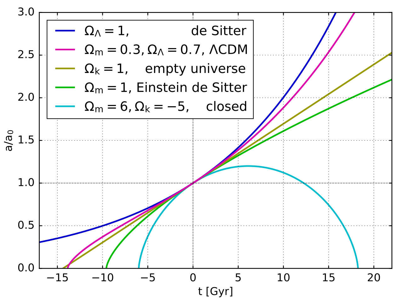
Plot of the evolution of the size of the universe (scale parameter
a
) over time (in billion years, Gyr). Different models are shown, which are all solutions to the
Friedmann equations
with different parameters. The evolution is governed by the equation
Here
is the radiation density,
the matter density,
the curvature parameter and
the dark energy, all normalized such that
represents the fact that today's expansion rate is
.
|
| Date | |
| Source | Own work |
| Author | Geek3 |
| SVG development |
This plot was created with
mplwp
, the
Matplotlib
extension for Wikipedia plots.
|
| Source code |
Python code#!/usr/bin/python
# -*- coding: utf8 -*-
import matplotlib.pyplot as plt
import matplotlib as mpl
import numpy as np
from math import *
code_website = 'http://commons.wikimedia.org/wiki/User:Geek3/mplwp'
try:
import mplwp
except ImportError, er:
print 'ImportError:', er
print 'You need to download mplwp.py from', code_website
exit(1)
name = 'mplwp_universe_scale_evolution.svg'
fig = mplwp.fig_standard(mpl)
fig.set_size_inches(600 / 72.0, 450 / 72.0)
mplwp.set_bordersize(fig, 58.5, 16.5, 16.5, 44.5)
xlim = -17, 22; fig.gca().set_xlim(xlim)
ylim = 0, 3; fig.gca().set_ylim(ylim)
mplwp.mark_axeszero(fig.gca(), y0=1)
import scipy.optimize as op
from scipy.integrate import odeint
tH = 978. / 68. # Hubble time in Gyr
def Hubble(a, matter, rad, k, darkE):
# the Friedman equation gives the relative expansion rate
a = a[0]
if a <= 0: return 0.
r = rad / a**4 + matter / a**3 + k / a**2 + darkE
if r < 0: return 0.
return sqrt(r) / tH
def scale(t, matter, rad, k, darkE):
return odeint(lambda a, t: a*Hubble(a, matter, rad, k, darkE), 1., [0, t])
def scaled_closed_matteronly(t, m):
# analytic solution for matter m > 1, rad=0, darkE=0
t0 = acos(2./m-1) * 0.5 * m / (m-1)**1.5 - 1. / (m-1)
try: psi = op.brentq(lambda p: (p - sin(p))*m/2./(m-1)**1.5
- t/tH - t0, 0, 2 * pi)
except Exception: psi=0
a = (1.0 - cos(psi)) * m * 0.5 / (m-1.)
return a
# De Sitter http://en.wikipedia.org/wiki/De_Sitter_universe
matter=0; rad=0; k=0; darkE=1
t = np.linspace(xlim[0], xlim[-1], 5001)
a = [scale(tt, matter, rad, k, darkE)[1,0] for tt in t]
plt.plot(t, a, zorder=-2,
label=ur'$\Omega_\Lambda=1$, de Sitter')
# Standard Lambda-CDM https://en.wikipedia.org/wiki/Lambda-CDM_model
matter=0.3; rad=0.; k=0; darkE=0.7
t0 = op.brentq(lambda t: scale(t, matter, rad, k, darkE)[1,0], -20, 0)
t = np.linspace(t0, xlim[-1], 5001)
a = [scale(tt, matter, rad, k, darkE)[1,0] for tt in t]
plt.plot(t, a, zorder=-1,
label=ur'$\Omega_m=0.\!3,\Omega_\Lambda=0.\!7$, $\Lambda$CDM')
# Empty universe
matter=0; rad=0; k=1; darkE=0
t0 = op.brentq(lambda t: scale(t, matter, rad, k, darkE)[1,0], -20, 0)
t = np.linspace(t0, xlim[-1], 5001)
a = [scale(tt, matter, rad, k, darkE)[1,0] for tt in t]
plt.plot(t, a, label=ur'$\Omega_k=1$, empty universe', zorder=-3)
'''
# Open Friedmann
matter=0.5; rad=0.; k=0.5; darkE=0
t0 = op.brentq(lambda t: scale(t, matter, rad, k, darkE)[1,0], -20, 0)
t = np.linspace(t0, xlim[-1], 5001)
a = [scale(tt, matter, rad, k, darkE)[1,0] for tt in t]
plt.plot(t, a, label=ur'$\Omega_m=0.\!5, \Omega_k=0.5$')
'''
# Einstein de Sitter http://en.wikipedia.org/wiki/Einstein–de_Sitter_universe
matter=1.; rad=0.; k=0; darkE=0
t0 = op.brentq(lambda t: scale(t, matter, rad, k, darkE)[1,0], -20, 0)
t = np.linspace(t0, xlim[-1], 5001)
a = [scale(tt, matter, rad, k, darkE)[1,0] for tt in t]
plt.plot(t, a, label=ur'$\Omega_m=1$, Einstein de Sitter', zorder=-4)
'''
# Radiation dominated
matter=0; rad=1.; k=0; darkE=0
t0 = op.brentq(lambda t: scale(t, matter, rad, k, darkE)[1,0], -20, 0)
t = np.linspace(t0, xlim[-1], 5001)
a = [scale(tt, matter, rad, k, darkE)[1,0] for tt in t]
plt.plot(t, a, label=ur'$\Omega_r=1$')
'''
# Closed Friedmann
matter=6; rad=0.; k=-5; darkE=0
t0 = op.brentq(lambda t: scaled_closed_matteronly(t, matter)-1e-9, -20, 0)
t1 = op.brentq(lambda t: scaled_closed_matteronly(t, matter)-1e-9, 0, 20)
t = np.linspace(t0, t1, 5001)
a = [scaled_closed_matteronly(tt, matter) for tt in t]
plt.plot(t, a, label=ur'$\Omega_m=6, \Omega_k=\u22125$, closed', zorder=-5)
plt.xlabel('t [Gyr]')
plt.ylabel(ur'$a/a_0$')
plt.legend(loc='upper left', borderaxespad=0.6, handletextpad=0.5)
plt.savefig(name)
mplwp.postprocess(name)
|


Licensing
I, the copyright holder of this work, hereby publish it under the following license:
This file is licensed under the
Creative Commons
Attribution-Share Alike 4.0 International
license.
-
You are free:
- to share – to copy, distribute and transmit the work
- to remix – to adapt the work
-
Under the following conditions:
- attribution – You must give appropriate credit, provide a link to the license, and indicate if changes were made. You may do so in any reasonable manner, but not in any way that suggests the licensor endorses you or your use.
- share alike – If you remix, transform, or build upon the material, you must distribute your contributions under the same or compatible license as the original.