Quartiles

Quartile

Quartile

Statistic which divides data into four same-sized parts for analysis


In statistics, quartiles are a type of quantiles which divide the number of data points into four parts, or quarters, of more-or-less equal size. The data must be ordered from smallest to largest to compute quartiles; as such, quartiles are a form of order statistic. The three quartiles, resulting in four data divisions, are as follows:

  • The first quartile (Q1) is defined as the 25th percentile where lowest 25% data is below this point. It is also known as the lower quartile.
  • The second quartile (Q2) is the median of a data set; thus 50% of the data lies below this point.
  • The third quartile (Q3) is the 75th percentile where lowest 75% data is below this point. It is known as the upper quartile, as 75% of the data lies below this point.[1]

Along with the minimum and maximum of the data (which are also quartiles), the three quartiles described above provide a five-number summary of the data. This summary is important in statistics because it provides information about both the center and the spread of the data. Knowing the lower and upper quartile provides information on how big the spread is and if the dataset is skewed toward one side. Since quartiles divide the number of data points evenly, the range is generally not the same between adjacent quartiles (i.e. usually (Q3 - Q2) ≠ (Q2 - Q1)). Interquartile range (IQR) is defined as the difference between the 75th and 25th percentiles or Q3 - Q1. While the maximum and minimum also show the spread of the data, the upper and lower quartiles can provide more detailed information on the location of specific data points, the presence of outliers in the data, and the difference in spread between the middle 50% of the data and the outer data points.[2]

Definitions

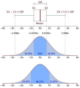
Boxplot (with quartiles and an interquartile range) and a probability density function (pdf) of a normal N(0,1σ2) population
More information Symbol, Names ...

Computing methods

Discrete distributions

For discrete distributions, there is no universal agreement on selecting the quartile values.[3]

Method 1

  1. Use the median to divide the ordered data set into two-halves. The median becomes the second quartiles.
    • If there are an odd number of data points in the original ordered data set, do not include the median (the central value in the ordered list) in either half.
    • If there are an even number of data points in the original ordered data set, split this data set exactly in half.
  2. The lower quartile value is the median of the lower half of the data. The upper quartile value is the median of the upper half of the data.

This rule is employed by the TI-83 calculator boxplot and "1-Var Stats" functions.

Method 2

  1. Use the median to divide the ordered data set into two-halves. The median becomes the second quartiles.
    • If there are an odd number of data points in the original ordered data set, include the median (the central value in the ordered list) in both halves.
    • If there are an even number of data points in the original ordered data set, split this data set exactly in half.
  2. The lower quartile value is the median of the lower half of the data. The upper quartile value is the median of the upper half of the data.

The values found by this method are also known as "Tukey's hinges";[4] see also midhinge.

Method 3

  1. Use the median to divide the ordered data set into two-halves. The median becomes the second quartiles.
    1. If there are odd numbers of data points, then go to the next step.
    2. If there are even numbers of data points, then the Method 3 starts off the same as the Method 1 or the Method 2 above and you can choose to include or not include the median as a new datapoint. If you choose to include the median as the new datapoint, then proceed to the step 2 or 3 below because you now have an odd number of datapoints. If you do not choose the median as the new data point, then continue the Method 1 or 2 where you have started.
  2. If there are (4n+1) data points, then the lower quartile is 25% of the nth data value plus 75% of the (n+1)th data value; the upper quartile is 75% of the (3n+1)th data point plus 25% of the (3n+2)th data point.
  3. If there are (4n+3) data points, then the lower quartile is 75% of the (n+1)th data value plus 25% of the (n+2)th data value; the upper quartile is 25% of the (3n+2)th data point plus 75% of the (3n+3)th data point.

Method 4

If we have an ordered dataset , then we can interpolate between data points to find the th empirical quantile if is in the quantile. If we denote the integer part of a number by , then the empirical quantile function is given by,

,

where and .[1]

To find the first, second, and third quartiles of the dataset we would evaluate , , and respectively.

Example 1

Ordered Data Set (of an odd number of data points): 6, 7, 15, 36, 39, 40, 41, 42, 43, 47, 49.

The bold number (40) is the median splitting the data set into two halves with equal number of data points.

More information Method 1, Method 2 ...

Example 2

Ordered Data Set (of an even number of data points): 7, 15, 36, 39, 40, 41.

The bold numbers (36, 39) are used to calculate the median as their average. As there are an even number of data points, the first three methods all give the same results. (The Method 3 is executed such that the median is not chosen as a new data point and the Method 1 started.)

More information Method 1, Method 2 ...

Continuous probability distributions

Quartiles on a cumulative distribution function of a normal distribution

If we define a continuous probability distributions as where is a real valued random variable, its cumulative distribution function (CDF) is given by

.[1]

The CDF gives the probability that the random variable is less than or equal to the value . Therefore, the first quartile is the value of when , the second quartile is when , and the third quartile is when .[5] The values of can be found with the quantile function where for the first quartile, for the second quartile, and for the third quartile. The quantile function is the inverse of the cumulative distribution function if the cumulative distribution function is monotonically increasing because the one-to-one correspondence between the input and output of the cumulative distribution function holds.

Outliers

There are methods by which to check for outliers in the discipline of statistics and statistical analysis. Outliers could be a result from a shift in the location (mean) or in the scale (variability) of the process of interest.[6] Outliers could also be evidence of a sample population that has a non-normal distribution or of a contaminated population data set. Consequently, as is the basic idea of descriptive statistics, when encountering an outlier, we have to explain this value by further analysis of the cause or origin of the outlier. In cases of extreme observations, which are not an infrequent occurrence, the typical values must be analyzed. The Interquartile Range (IQR), defined as the difference between the upper and lower quartiles (), may be used to characterize the data when there may be extremities that skew the data; the interquartile range is a relatively robust statistic (also sometimes called "resistance") compared to the range and standard deviation. There is also a mathematical method to check for outliers and determining "fences", upper and lower limits from which to check for outliers.

After determining the first (lower) and third (upper) quartiles ( and respectively) and the interquartile range () as outlined above, then fences are calculated using the following formula:

Boxplot Diagram with Outliers

The lower fence is the "lower limit" and the upper fence is the "upper limit" of data, and any data lying outside these defined bounds can be considered an outlier. The fences provide a guideline by which to define an outlier, which may be defined in other ways. The fences define a "range" outside which an outlier exists; a way to picture this is a boundary of a fence. It is common for the lower and upper fences along with the outliers to be represented by a boxplot. For the boxplot shown on the right, only the vertical heights correspond to the visualized data set while horizontal width of the box is irrelevant. Outliers located outside the fences in a boxplot can be marked as any choice of symbol, such as an "x" or "o". The fences are sometimes also referred to as "whiskers" while the entire plot visual is called a "box-and-whisker" plot.

When spotting an outlier in the data set by calculating the interquartile ranges and boxplot features, it might be easy to mistakenly view it as evidence that the population is non-normal or that the sample is contaminated. However, this method should not take place of a hypothesis test for determining normality of the population. The significance of the outliers varies depending on the sample size. If the sample is small, then it is more probable to get interquartile ranges that are unrepresentatively small, leading to narrower fences. Therefore, it would be more likely to find data that are marked as outliers.[7]

Computer software for quartiles

More information Environment, Function ...

Excel

The Excel function QUARTILE(array, quart) provides the desired quartile value for a given array of data, using Method 3 from above. In the QUARTILE function (a legacy function from Excel 2007 or earlier, giving the same output of the function QUARTILE.INC), array is the dataset of numbers that is being analyzed and quart is any of the following 5 values depending on which quartile is being calculated. [8]

More information Quart, Output QUARTILE Value ...

MATLAB

In order to calculate quartiles in Matlab, the function quantile(A,p) can be used. Where A is the vector of data being analyzed and p is the percentage that relates to the quartiles as stated below. [9]

More information p, Output QUARTILE Value ...

See also


References

  1. Dekking, Michel (2005). A modern introduction to probability and statistics: understanding why and how. London: Springer. pp. 236-238. ISBN 978-1-85233-896-1. OCLC 262680588.
  2. Knoch, Jessica (February 23, 2018). "How are Quartiles Used in Statistics?". Magoosh. Archived from the original on December 10, 2019. Retrieved February 24, 2023.
  3. Hyndman, Rob J; Fan, Yanan (November 1996). "Sample quantiles in statistical packages". American Statistician. 50 (4): 361–365. doi:10.2307/2684934. JSTOR 2684934.
  4. Walfish, Steven (November 2006). "A Review of Statistical Outlier Method". Pharmaceutical Technology.
  5. Dawson, Robert (July 1, 2011). "How Significant is a Boxplot Outlier?". Journal of Statistics Education. 19 (2). doi:10.1080/10691898.2011.11889610.
  6. "How to use the Excel QUARTILE function | Exceljet". exceljet.net. Retrieved December 11, 2019.
  7. "Quantiles of a data set – MATLAB quantile". www.mathworks.com. Retrieved December 11, 2019.

Share this article:

This article uses material from the Wikipedia article Quartiles, and is written by contributors. Text is available under a CC BY-SA 4.0 International License; additional terms may apply. Images, videos and audio are available under their respective licenses.